...
Simple functions of one variable can be graphed in three ways:
Typing and then the equation

Typing the equation
Typing and then the equation
Mathinline body --uriencoded--x%5e2 Typing
and then the equationMathinline body y= Mathinline body --uriencoded--x%5e3 Typing
and then the equationMathinline body f(x)= Mathinline body --uriencoded--\frac%7Bx%5e2%7D%7B7%7D 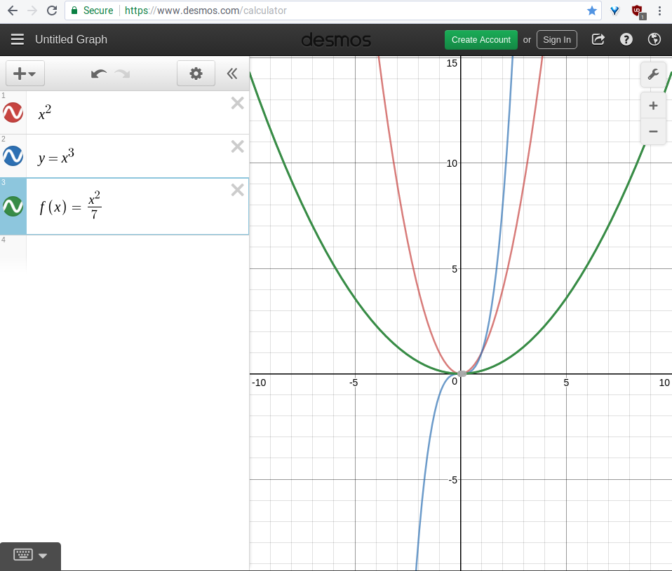
Functions can be hidden from the graph by clicking the colored circle to the left of their equation.
Functions can be functions of other functions. For example:
...
x^{2}}{\displaystyleMathinline body --uriencoded-- f(x)= x%5e%7B2%7D
}Mathinline body g(x)=f(x+1)
Functions can be graphed with x in terms of y: {\displaystyle x={\sqrt {1-y^{2}}}}
...
Functions can be of multiple variables. For example, {\displaystyle
| Mathinline | ||
|---|---|---|
|
|
| Mathinline | ||
|---|---|---|
|
Parametric Equations
In Desmos you can graph parametric equations. The standard form of this is {\displaystyle (f(t),g(t))}. For example, {\displaystyle (sin(2t),cos(3t))}. It is necessary to use the variable {\displaystyle t} in order for the equation to be interpreted as a parametric equation.
...
Input | Result | Explanation | ||||
|---|---|---|---|---|---|---|
exp(x) | exp(x) |
| ||||
ln(x) | ln(x) | The natural log of x | ||||
log(x) | log(x) | The log (base 10) of x | ||||
log_n(x) | The log (base n) of x | |||||
x^n | x to the nth power | |||||
sqrtx |
| The square root of x | ||||
nthrootx |
| The generalized root function. |
...
Input | Result | Explanation | |||||
|---|---|---|---|---|---|---|---|
sum |
| The summation operator | |||||
prod |
| The product operator. | |||||
int |
| The integral operator. | |||||
d/dx |
| The differential operator. Can be used on functions. |
...
Function | Explanation | ||||
|---|---|---|---|---|---|
total() | Sum of all elements in a list | ||||
length() | Number of elements in a list | ||||
mean() | Mean of a list | ||||
median() | Median element in a list | ||||
min() | Minimum element in a list | ||||
max() | Maximum element in a list | ||||
quantile() | The quantile function | ||||
mad() | Mean absolute deviation | ||||
stdev() | Sample standard deviation | ||||
stdevp() | Population standard deviation | ||||
var() | Variance | ||||
cov() | Covariance | ||||
corr() | Pearson correlation coefficient of two lists | ||||
nCr() | Number of combinations | ||||
nPr() | Number of permutations | ||||
| Factorial |
Miscellaneous Functions
Input | Explanation | ||||
|---|---|---|---|---|---|
lcm(a,b) | The least common multiple of a and b | ||||
gcd(a,b) | The greatest common denominator of a and b | ||||
mod(a, b) | The modulo function | ||||
ceil(x) | The closest integer above x | ||||
floor(x) | The closest integer below x | ||||
round(x) | The closest integer to x | ||||
sign(x) | The sign of x | ||||
abs(x) | The absolute value function | ||||
| The absolute value operator | ||||
a%b | a percent of b |
...
To do this, click the wrench in the top right corner (graph settings). After this, a window will appear. In this window, there are inequalities for {\displaystyle x} and {\displaystyle y} ({\displaystyle
| Mathinline | ||
|---|---|---|
|
| Mathinline | ||
|---|---|---|
|
| Mathinline | ||
|---|---|---|
|
| Mathinline | ||
|---|---|---|
|
| Mathinline | ||
|---|---|---|
|
| Mathinline | ||
|---|---|---|
|
...
Changing line colors/styles
...