| Info |
|---|
Desmos is a free online graphing calculator. Some classes at NCSSM require its usage, but it is a tool that any student of mathematics will appreciate. Here are enumerated some of the simple and complex functions of the software you might find useful. If this page is not sufficient, see the Desmos user guide for more information. Below is a brief description of how to effectively use the Desmos online graphing calculator. Click the images to enlarge them. |
| Table of Contents |
|---|
Graphing
Functions
Simple functions of one variable can be graphed in three ways:
Typing the equation
Mathinline body --uriencoded--x%5e2 Typing
and then the equationMathinline body y= Mathinline body --uriencoded--x%5e3 Typing
and then the equationMathinline body f(x)= Mathinline body --uriencoded--\frac%7Bx%5e2%7D%7B7%7D 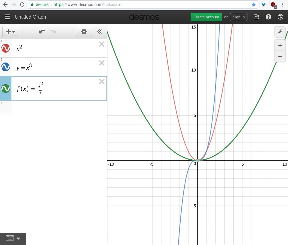
Functions can be hidden from the graph by clicking the colored circle to the left of their equation.
Functions can be functions of other functions. For example:
Mathinline body --uriencoded-- f(x)=x%5e%7B2%7D Mathinline body g(x)=f(x+1)
Functions can be graphed with
| Mathinline | ||
|---|---|---|
|
| Mathinline | ||
|---|---|---|
|
| Mathinline | ||
|---|---|---|
|
Functions can be of multiple variables. For example,
| Mathinline | ||
|---|---|---|
|
| Mathinline | ||
|---|---|---|
|
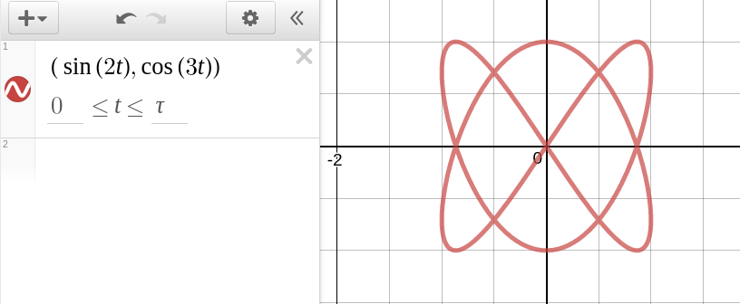
Parametric Equations
In Desmos you can graph parametric equations. The standard form of this is
| Mathinline | ||
|---|---|---|
|
| Mathinline | ||
|---|---|---|
|
| Mathinline | ||
|---|---|---|
|
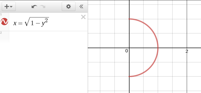
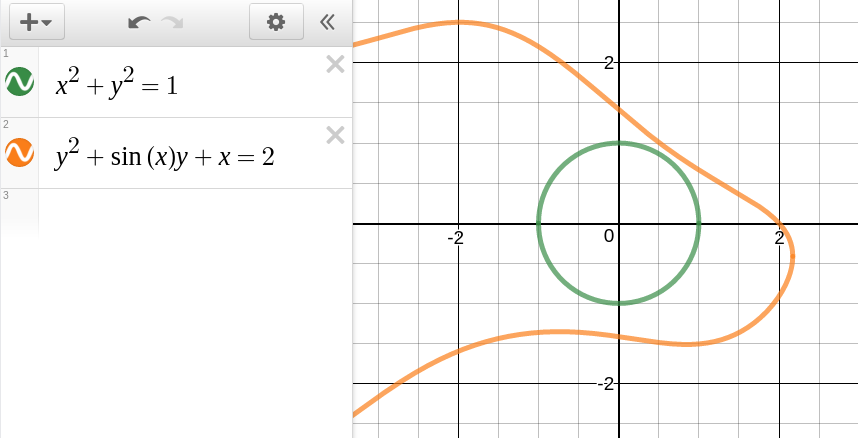
Implicit Functions
Solutions of equations involving
| Mathinline | ||
|---|---|---|
|
| Mathinline | ||
|---|---|---|
|
| Mathinline | ||
|---|---|---|
|
| Mathinline | ||
|---|---|---|
|
Points and Tables
Points can be graphed in two ways. One way is by clicking the plus in the upper left, and then selecting table. Points can be added manually, or pasted in from an outside source, such as Logger Pro. The points will appear on the graph, but the viewport will not scale to accommodate them. To do this, see Resizing the viewport.
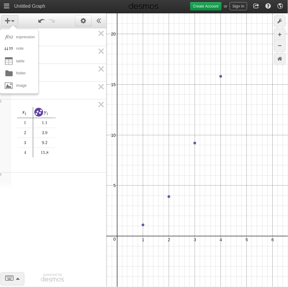
For an interactive demonstration of how to add points to a table, click here.
The other way to graph points is by adding them in the form
| Mathinline | ||
|---|---|---|
|
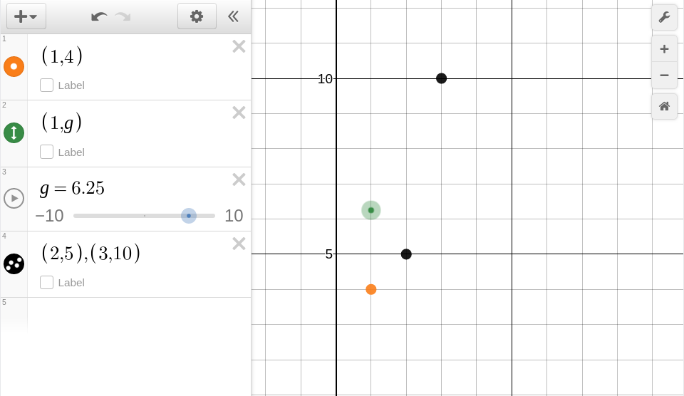
Movable points can be graphed by setting one or both of the parameters to variables:
| Mathinline | ||
|---|---|---|
|
| Mathinline | ||
|---|---|---|
|
You can add multiple points by separating them with commas, like so:
| Mathinline | ||
|---|---|---|
|
Variables and Sliders
Sometimes, for example, when looking for the value of a constant or seeing how a function reacts to a change in one of its parts, it is useful to use a slider. Sliders represent a named variable.
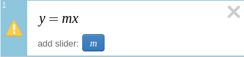
To add a slider, write a function with a free variable, such as
| Mathinline | ||
|---|---|---|
|
Another way to add variables is to type the variable letter, "=", and then a starting value. For example,
| Mathinline | ||
|---|---|---|
|
Clicking on either of the constraints of a slider allows you to set the minimum, maximum, and step values.
For an interactive demonstration of how to use sliders, click here.
Regressions (Linear, quadratic, etc)
Performing regression analysis of data in Desmos is simple. First, enter the data points in a table as explained in Graphing Points.
Next, decide on the type of regression. If you want to do a linear regression, the equation would take the form
...
| Mathinline | ||
|---|---|---|
|
...
...
| Mathinline | ||
|---|---|---|
|
...
...
as
| Mathinline | ||
|---|---|---|
|
After you have decided the form your equation should take, substitute "
...
| Mathinline | ||
|---|---|---|
|
| Mathinline | ||
|---|---|---|
|
| Mathinline | ||
|---|---|---|
|
| Mathinline | ||
|---|---|---|
|
| Mathinline | ||
|---|---|---|
|
| Mathinline | ||
|---|---|---|
|
...
| Mathinline | ||
|---|---|---|
|
...
|
...
...
| Mathinline | ||
|---|---|---|
|
...
| Mathinline | ||
|---|---|---|
|
| Mathinline | ||
|---|---|---|
|
...
| Mathinline | ||
|---|---|---|
|
...
|
| Mathinline | ||
|---|---|---|
|
...
|
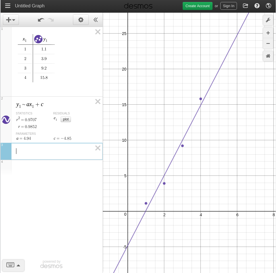
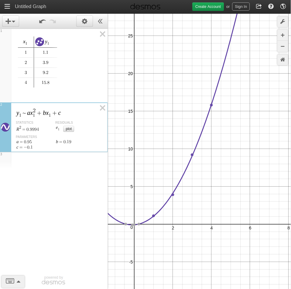
Desmos will find the best constants that fit the points and function you put in. The value of each constant is shown under your function entry. As you can see, the function it finds is not always in the correct form. (This is because you provide the form, Desmos only finds the best values for the free variables that it can.) Above, the same points were used, but a line and a parabola were both found. The equation you get out is only as good as the equation form you put in.
One way to check whether the form of the function is correct is to plot the residuals, and see if there is a pattern. If you see a clear trend, such as the residuals moving in a straight line, parabola, or sinusoidal curve, you know you chose the wrong function to model your data, even if the r-value is small.
See Desmos regressions tour for an interactive demonstration for plotting regressions.
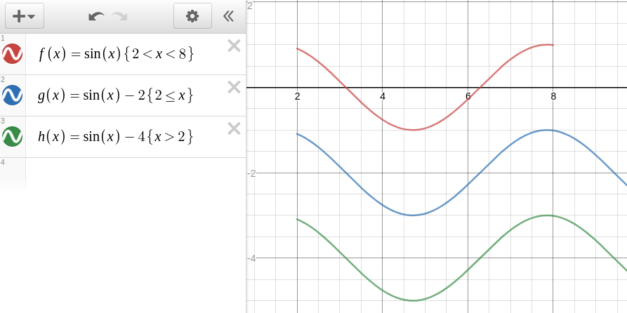
Restrictions
It can be useful to restrict the domain or range of a function. To do this, add a restriction of the form
...
| Mathinline | ||
|---|---|---|
|
...
|
...
|
...
| Mathinline | ||
|---|---|---|
|
...
|
...
|
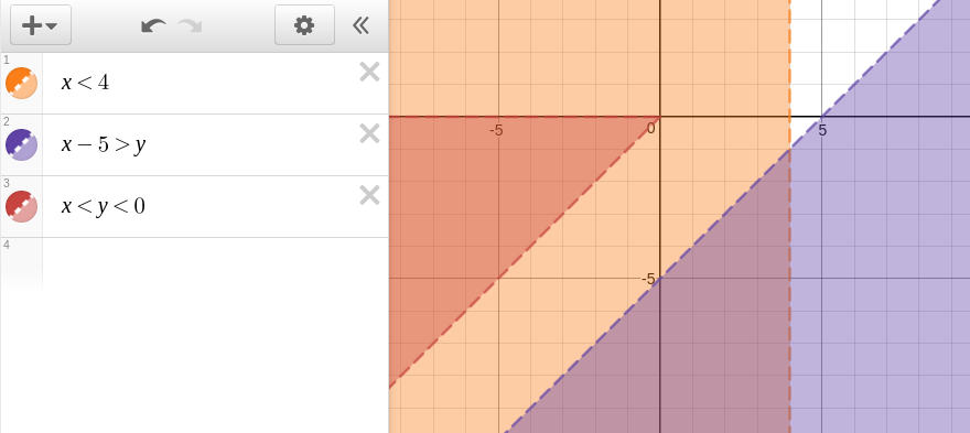
Inequalities
Desmos also has the capability to graph inequalities. Simple inequalities are easy: type an expression followed by a comparison sign (e.g.
...
| Mathinline | ||
|---|---|---|
|
| Mathinline | ||
|---|---|---|
|
...
| Mathinline | ||
|---|---|---|
|
...
| Mathinline | ||
|---|---|---|
|
You can also use this on functions you define. For example, say you're modeling compound interest, and want to set up an inequality for the space under the curve. To do this, define a function for amount given time,
...
| Mathinline | ||
|---|---|---|
|
...
...
| Mathinline | ||
|---|---|---|
|
...
...
| Mathinline | ||
|---|---|---|
|
| Mathinline | ||
|---|---|---|
|
| Mathinline | ||
|---|---|---|
|
| Mathinline | ||
|---|---|---|
|
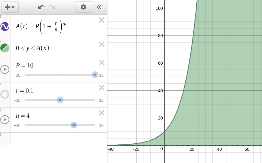
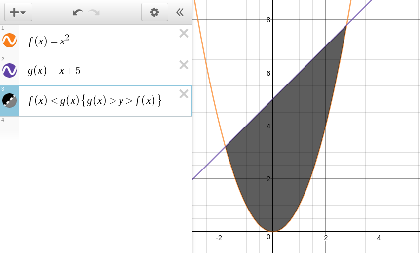
We can use this powerful tool in tandem with restrictions. To graph the area between functions
...
| Mathinline | ||
|---|---|---|
|
...
| Mathinline | ||
|---|---|---|
|
...
...
| Mathinline | ||
|---|---|---|
|
...
|
...
|
Built-in Functions and Symbols
Desmos comes with many built in functions and symbols. Here are some of the documented and undocumented ones. Most of these can be accessed by opening the keyboard and clicking "functions".
Variables
Input | Result | Explanation | ||||
|---|---|---|---|---|---|---|
theta |
| A variable, like |
Constants
Input | Result | Explanation | |||||
|---|---|---|---|---|---|---|---|
pi |
| The constant 3.14... | |||||
tau |
...
| The constant 6.28... | |||||
e |
...
| The constant 2.71... |
Exponent and Log Functions
Input | Result | Explanation | ||||
|---|---|---|---|---|---|---|
exp(x) | exp(x) |
| ||||
ln(x) | ln(x) | The natural log of x | ||||
log(x) | log(x) | The log (base 10) of x | ||||
log_n(x) |
...
| The log (base n) of x | ||
x^n |
...
| x to the nth power | |||||
sqrtx |
| The square root of x | ||||
nthrootx |
| The generalized root function. |
Precalculus and Calculus Functions
Input | Result | Explanation | |||||
|---|---|---|---|---|---|---|---|
sum |
| The summation operator | |||||
prod |
| The product operator. | |||||
int |
| The integral operator. | |||||
d/dx |
| The differential operator. Can be used on functions. |
Trig Functions
sin(x) | arcsin(x) or
| sinh(x) | ||||
cos(x) | arccos(x) or
| cosh(x) | ||||
tan(x) | arctan(x) or
| tanh(x) | ||||
sec(x) | arcsec(x) or
| sech(x) | ||||
csc(x) | arccsc(x) or
| csch(x) | ||||
cot(x) | arccot(x) or
| coth(x) |
Stats and Probability Functions
Function | Explanation | ||||
|---|---|---|---|---|---|
total() | Sum of all elements in a list | ||||
length() | Number of elements in a list | ||||
mean() | Mean of a list | ||||
median() | Median element in a list | ||||
min() | Minimum element in a list | ||||
max() | Maximum element in a list | ||||
quantile() | The quantile function | ||||
mad() | Mean absolute deviation | ||||
stdev() | Sample standard deviation | ||||
stdevp() | Population standard deviation | ||||
var() | Variance | ||||
cov() | Covariance | ||||
corr() | Pearson correlation coefficient of two lists | ||||
nCr() | Number of combinations | ||||
nPr() | Number of permutations | ||||
| Factorial |
Miscellaneous Functions
Input | Explanation | ||||
|---|---|---|---|---|---|
lcm(a,b) | The least common multiple of a and b | ||||
gcd(a,b) | The greatest common denominator of a and b | ||||
mod(a, b) | The modulo function | ||||
ceil(x) | The closest integer above x | ||||
floor(x) | The closest integer below x | ||||
round(x) | The closest integer to x | ||||
sign(x) | The sign of x | ||||
abs(x) | The absolute value function | ||||
| The absolute value operator | ||||
a%b | a percent of b |
Making graphs easier to read
Resizing the viewport
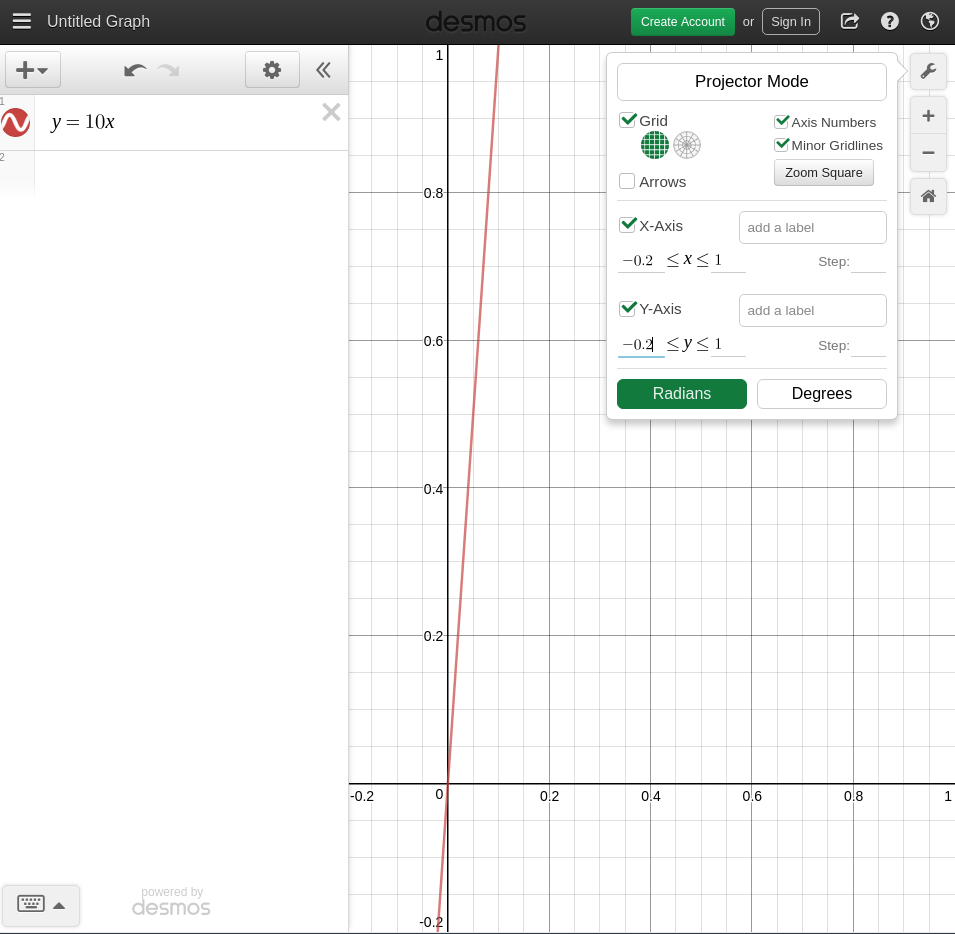
The viewport (the section of the coordinate plane visible onscreen) can be resized to give a better view of your data and functions. One way to resize it is to scroll down to zoom out, and up to zoom in, and to click and drag to move. This method, however, keeps the ratio of the domain and range constant. Sometimes it is useful to be able to zoom to an arbitrary window.
To do this, click the wrench in the top right corner (graph settings). After this, a window will appear. In this window, there are inequalities for
| Mathinline | ||
|---|---|---|
|
| Mathinline | ||
|---|---|---|
|
| Mathinline | ||
|---|---|---|
|
| Mathinline | ||
|---|---|---|
|
| Mathinline | ||
|---|---|---|
|
| Mathinline | ||
|---|---|---|
|
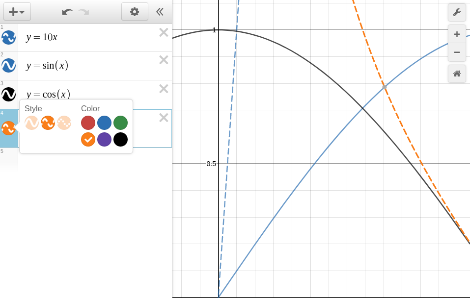
Changing line colors/styles
If you have many functions graphed, it can be useful to change their appearance. To do this, perform a long left click on the icon to the left of the function definition. From here, you may change the style to dashed, dotted, or unbroken, and the color to one of six options.
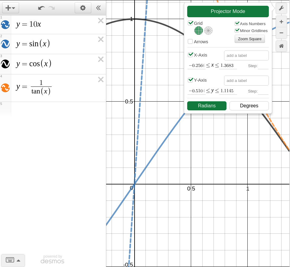
Projector mode
When saving images for reports or projects, it can be useful to have thicker, fuller lines and larger text. To enable this, go to graph settings and enable "Projector Mode".
Related articles
| Filter by label (Content by label) | ||||||||||||||||||
|---|---|---|---|---|---|---|---|---|---|---|---|---|---|---|---|---|---|---|
|
...
| hidden | true |
|---|
...